Compare samplers

In this notebook, we’ll compare the different samplers implemented in Bilby on a simple linear regression problem.

This is not an exhaustive set of the implemented samplers, nor of the settings available for each sampler.

Setup

import bilby
import numpy as np
import matplotlib.pyplot as plt
from bilby.core.utils import random

# Sets seed of bilby's generator "rng" to "123" to ensure reproducibility
random.seed(123)

%matplotlib inline

label = "linear_regression"
outdir = "outdir"
bilby.utils.check_directory_exists_and_if_not_mkdir(outdir)

Define our model

Here our model is a simple linear fit to some quantity \(y = m x + c\).

def model(x, m, c):
    return x * m + c

Simulate data

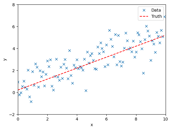
We simulate observational data. We assume some uncertainty in the observations and so perturb the observations from the truth.

injection_parameters = dict(m=0.5, c=0.2)

sampling_frequency = 10
time_duration = 10
time = np.arange(0, time_duration, 1 / sampling_frequency)
N = len(time)
sigma = random.rng.normal(1, 0.01, N)
data = model(time, **injection_parameters) + random.rng.normal(0, sigma, N)

fig, ax = plt.subplots()
ax.plot(time, data, "x", label="Data")
ax.plot(time, model(time, **injection_parameters), "--r", label="Truth")
ax.set_xlim(0, 10)
ax.set_ylim(-2, 8)
ax.set_xlabel("x")
ax.set_ylabel("y")
ax.legend()
plt.show()
plt.close()

Define the likelihood and prior

For any Bayesian calculation we need a likelihood and a prior.

In this case, we take a GausianLikelihood as we assume the uncertainty on the data is normally distributed.

For both of our parameters we take uniform priors.

likelihood = bilby.likelihood.GaussianLikelihood(time, data, model, sigma)

priors = bilby.core.prior.PriorDict()
priors["m"] = bilby.core.prior.Uniform(0, 5, "m")
priors["c"] = bilby.core.prior.Uniform(-2, 2, "c")

Run the samplers and compare the inferred posteriors

We’ll use four of the implemented samplers.

For each one we specify a set of parameters.

Bilby/the underlying samplers produce quite a lot of output while the samplers are running so we will suppress as many of these as possible.

After running the analysis, we print a final summary for each of the samplers.

samplers = dict(
    bilby_mcmc=dict(
        nsamples=1000,
        L1steps=20,
        ntemps=10,
        printdt=10,
    ),
    dynesty=dict(npoints=500, sample="acceptance-walk", naccept=20),
    nessai=dict(nlive=500),
    nestle=dict(nlive=500),
    emcee=dict(nwalkers=20, iterations=500),
    zeus=dict(nwalkers=20, iterations=500),
)

results = dict()

bilby.core.utils.logger.setLevel("ERROR")

for sampler in samplers:
    print(f"Running sampler: {sampler}")
    result = bilby.core.sampler.run_sampler(
        likelihood,
        priors=priors,
        sampler=sampler,
        label=sampler,
        resume=False,
        clean=True,
        verbose=False,
        **samplers[sampler]
    )
    results[sampler] = result

Running sampler: bilby_mcmc
Running sampler: dynesty
Running sampler: nessai

/opt/conda/envs/python312/lib/python3.12/site-packages/nessai/gw/__init__.py:12: FutureWarning: The `nessai.gw` module will be deprecated in the next release in favour of the nessai-gw package. This packages provides the same functionality as`nessai.gw` via the plugin interface.For more details, see: https://github.com/mj-will/nessai-gw
  warnings.warn(

Running sampler: nestle

Running sampler: emcee
Running sampler: zeus

Initialising ensemble of 20 walkers...
Sampling progress : 100%|██████████| 500/500 [00:04<00:00, 119.68it/s]

print("=" * 40)
for sampler in results:
    print(sampler)
    print("=" * 40)
    print(results[sampler])
    print("=" * 40)

========================================
bilby_mcmc
========================================
nsamples: 2025
ln_noise_evidence:    nan
ln_evidence: -137.646 +/-  0.030
ln_bayes_factor:    nan +/-  0.030

========================================
dynesty
========================================
nsamples: 1314
ln_noise_evidence:    nan
ln_evidence: -140.456 +/-  0.134
ln_bayes_factor:    nan +/-  0.134

========================================
nessai
========================================
nsamples: 1328
ln_noise_evidence:    nan
ln_evidence: -140.432 +/-  0.107
ln_bayes_factor:    nan +/-  0.107

========================================
nestle
========================================
nsamples: 4327
ln_noise_evidence:    nan
ln_evidence: -140.525 +/-  0.108
ln_bayes_factor:    nan +/-  0.108

========================================
emcee
========================================
nsamples: 8500
ln_noise_evidence:    nan
ln_evidence:    nan +/-    nan
ln_bayes_factor:    nan +/-    nan

========================================
zeus
========================================
nsamples: 9820
ln_noise_evidence:    nan
ln_evidence:    nan +/-    nan
ln_bayes_factor:    nan +/-    nan

========================================

Make comparison plots

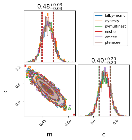
We will make two standard comparison plots.

In the first we plot the one- and two-dimensional marginal posterior distributions in a “corner” plot.

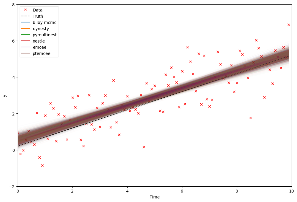
In the second, we show the inferred model that we are fitting along with the uncertainty by taking random draws from the posterior distribution. This kind of posterior predicitive plot is useful to identify model misspecification.

_ = bilby.core.result.plot_multiple(
    list(results.values()), labels=list(results.keys()), save=False
)
plt.show()
plt.close()

Found 'auto' as default backend, checking available backends
Matplotlib is available, defining as default backend
arviz_base 1.1.0 available, exposing its functions as part of the `arviz` namespace
arviz_stats 1.1.0 available, exposing its functions as part of the `arviz` namespace
arviz_plots 1.1.0 available, exposing its functions as part of the `arviz` namespace

fig, ax = plt.subplots(figsize=(12, 8))
ax.plot(time, data, "x", label="Data", color="r")
ax.plot(
    time, model(time, **injection_parameters), linestyle="--", color="k", label="Truth"
)

for jj, sampler in enumerate(samplers):
    result = results[sampler]
    samples = result.posterior[result.search_parameter_keys].sample(500)
    for ii in range(len(samples)):
        parameters = dict(samples.iloc[ii])
        plt.plot(time, model(time, **parameters), color=f"C{jj}", alpha=0.01)
    plt.axhline(-10, color=f"C{jj}", label=sampler.replace("_", " "))
ax.set_xlim(0, 10)
ax.set_ylim(-2, 8)
ax.set_xlabel("Time")
ax.set_ylabel("y")
ax.legend(loc="upper left")
plt.show()
plt.close()