! rm visualising_the_results/*

rm: cannot remove 'visualising_the_results/*': No such file or directory

Visualising the results

In this tutorial, we demonstrate the plotting tools built-in to bilby and how to extend them. First, we run a simple injection study and return the result object.

import bilby
import matplotlib.pyplot as plt

%matplotlib inline

duration = 4
sampling_frequency = 2048
outdir = "visualising_the_results"
label = "example"

injection_parameters = dict(
    mass_1=36.0,
    mass_2=29.0,
    a_1=0.4,
    a_2=0.3,
    tilt_1=0.5,
    tilt_2=1.0,
    phi_12=1.7,
    phi_jl=0.3,
    luminosity_distance=1000.0,
    theta_jn=0.4,
    phase=1.3,
    ra=1.375,
    dec=-1.2108,
    geocent_time=1126259642.413,
    psi=2.659,
)

# specify waveform arguments
waveform_arguments = dict(
    waveform_approximant="IMRPhenomXP",  # waveform approximant name
    reference_frequency=50.0,  # gravitational waveform reference frequency (Hz)
)

# set up the waveform generator
waveform_generator = bilby.gw.waveform_generator.WaveformGenerator(
    sampling_frequency=sampling_frequency,
    duration=duration,
    frequency_domain_source_model=bilby.gw.source.lal_binary_black_hole,
    parameters=injection_parameters,
    waveform_arguments=waveform_arguments,
)

ifos = bilby.gw.detector.InterferometerList(["H1", "L1"])
ifos.set_strain_data_from_power_spectral_densities(
    duration=duration,
    sampling_frequency=sampling_frequency,
    start_time=injection_parameters["geocent_time"] - 2,
)
_ = ifos.inject_signal(
    waveform_generator=waveform_generator, parameters=injection_parameters
)

/home/runner/work/bilby/bilby/.pixi/envs/documentation/lib/python3.13/site-packages/lalsimulation/lalsimulation.py:8: UserWarning: Wswiglal-redir-stdio:

SWIGLAL standard output/error redirection is enabled in IPython.
This may lead to performance penalties. To disable locally, use:

with lal.no_swig_redirect_standard_output_error():
    ...

To disable globally, use:

lal.swig_redirect_standard_output_error(False)

Note however that this will likely lead to error messages from
LAL functions being either misdirected or lost when called from
Jupyter notebooks.

To suppress this warning, use:

import warnings
warnings.filterwarnings("ignore", "Wswiglal-redir-stdio")
import lal

  import lal

# first, set up all priors to be equal to a delta function at their designated value
priors = bilby.gw.prior.BBHPriorDict(injection_parameters.copy())
# then, reset the priors on the masses and luminosity distance to conduct a search over these parameters
priors["mass_1"] = bilby.core.prior.Uniform(25, 40, "mass_1")
priors["mass_2"] = bilby.core.prior.Uniform(25, 40, "mass_2")
priors["luminosity_distance"] = bilby.core.prior.Uniform(
    400, 2000, "luminosity_distance"
)

# compute the likelihoods
likelihood = bilby.gw.likelihood.GravitationalWaveTransient(
    interferometers=ifos, waveform_generator=waveform_generator
)

Set up the sampling

For this case we use the dynesty sampler with 100 live points and the uniform sampling method. While these settings are sufficient for this simple, three-dimensional problem, they often don’t work for more complex cases.

result = bilby.core.sampler.run_sampler(
    likelihood=likelihood,
    priors=priors,
    sampler="dynesty",
    npoints=100,
    injection_parameters=injection_parameters,
    outdir=outdir,
    label=label,
    sample="unif",
)

Corner plots

Now lets make some corner plots. You can easily generate a corner plot using result.plot_corner() like this:

result.plot_corner(save=False)
plt.show()
plt.close()

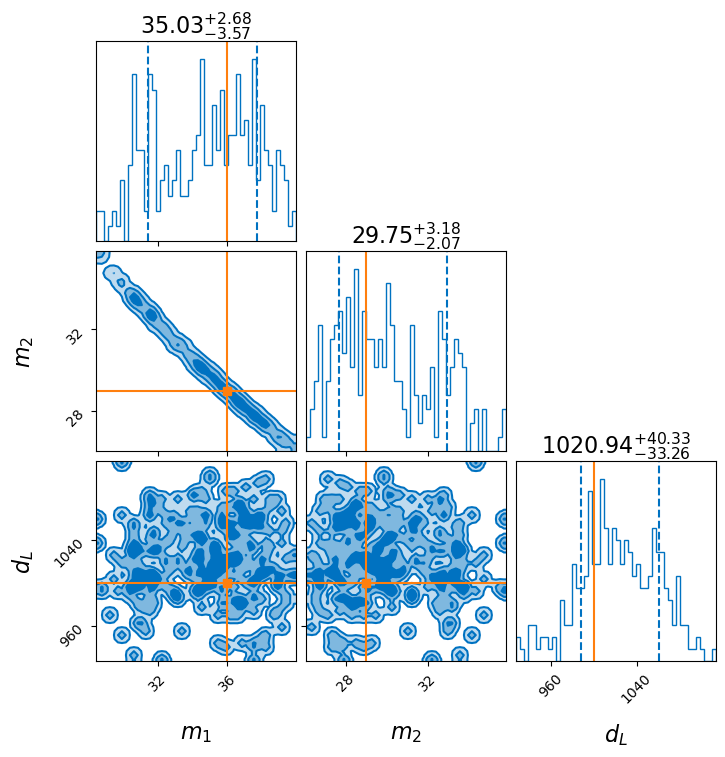
In a notebook, this figure will display. But by default the file is also saved to visualising_the_result/example_corner.png. If you change the label to something more descriptive then the example here will of course be replaced.

Waveform Reconstruction plot

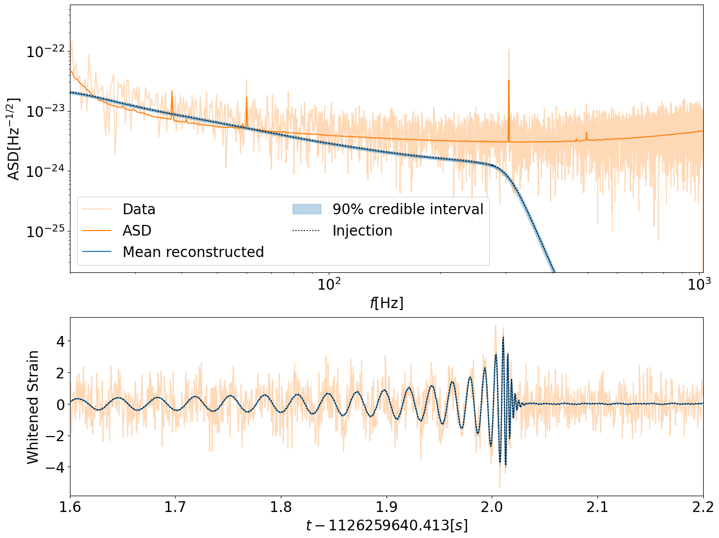
Some plots specific to compact binary coalescence parameter estimation results can be created by re-loading the result as a CBCResult:

from bilby.gw.result import CBCResult

cbc_result = CBCResult.from_json("visualising_the_results/example_result.json")
for ifo in ifos:
    cbc_result.plot_interferometer_waveform_posterior(
        interferometer=ifo, n_samples=500, save=False
    )
    plt.show()
    plt.close()

Marginal Distribution plots

These plots just show the 1D histograms for each parameter

result.plot_marginals()

Customizing corner plots

You may also want to plot a subset of the parameters, or perhaps add the injection_paramters as lines to check if you recovered them correctly. All this can be done through plot_corner. Under the hood, plot_corner uses corner, and all the keyword arguments passed to plot_corner are passed through.

Adding injection parameters to the plot

In the previous plot, you’ll notice bilby added the injection parameters to the plot by default. You can switch this off by setting truth=None when you call plot_corner. Or to add different injection parameters to the plot, just pass this as a keyword argument for truth. In this example, we just add a line for the luminosity distance by passing a dictionary of the value we want to display.

result.plot_corner(truth=dict(luminosity_distance=201))
plt.show()
plt.close()

Plot a subset of the corner plot

Or, to plot just a subset of parameters, just pass a list of the names you want.

result.plot_corner(
    parameters=["mass_1", "mass_2"], filename="{}/subset.png".format(outdir)
)
plt.show()
plt.close()

Notice here, we also passed in a keyword argument filename=, this overwrites the default filename and instead saves the file as visualising_the_results/subset.png. Useful if you want to create lots of different plots.

Alternative

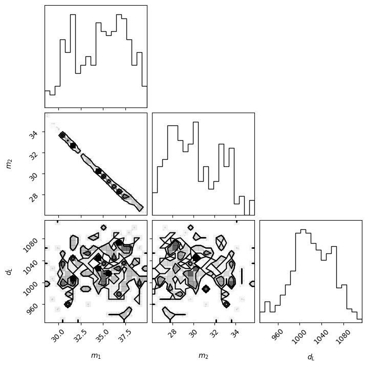
If you would prefer to do the plotting yourself, you can get hold of the samples and the ordering as follows and then plot with a different module. Here is an example using the corner package

import corner

samples = result.samples
labels = result.parameter_labels
fig = corner.corner(samples, labels=labels)
plt.show()
plt.close()

WARNING:root:Too few points to create valid contours
WARNING:root:Too few points to create valid contours